This is a post about a virtual work experience program I completed with Forage in their collaboration with ANZ, an Australian multinational banking and financial services company.
Overview
The virtual work experiences contain a series of resources and tasks designed to simulate the real-world experience. This task is based on a synthesised transaction dataset containing 3 months’ worth of transactions for 100 hypothetical customers. It contains purchases, recurring transactions, and salary transactions.
The dataset is designed to simulate realistic transaction behaviours that are observed in ANZ’s real transaction data, so many of the insights you can gather from the tasks below will be genuine.
This task will involve exploratory data analysis, feature engineering and predicting customers’ annual salary based on their transactions.
Have a look at this interactive data dashboard too. And if you would like to deep dive into the code, here is a link to the github repository.
Exploratory Data Analysis
The dataset given has 12 043 records with 23 columns.
<class 'pandas.core.frame.DataFrame'>
RangeIndex: 12043 entries, 0 to 12042
Data columns (total 23 columns):
 #   Column             Non-Null Count  Dtype
---  ------             --------------  -----
 0   status             12043 non-null  object
 1   card_present_flag  7717 non-null   float64
 2   bpay_biller_code   885 non-null    object
 3   account            12043 non-null  object
 4   currency           12043 non-null  object
 5   long_lat           12043 non-null  object
 6   txn_description    12043 non-null  object
 7   merchant_id        7717 non-null   object
 8   merchant_code      883 non-null    float64
 9   first_name         12043 non-null  object
 10  balance            12043 non-null  float64
 11  date               12043 non-null  datetime64[ns]
 12  gender             12043 non-null  object
 13  age                12043 non-null  int64
 14  merchant_suburb    7717 non-null   object
 15  merchant_state     7717 non-null   object
 16  extraction         12043 non-null  object
 17  amount             12043 non-null  float64
 18  transaction_id     12043 non-null  object
 19  country            12043 non-null  object
 20  customer_id        12043 non-null  object
 21  merchant_long_lat  7717 non-null   object
 22  movement           12043 non-null  object
dtypes: datetime64[ns](1), float64(4), int64(1), object(17)
memory usage: 2.1+ MB
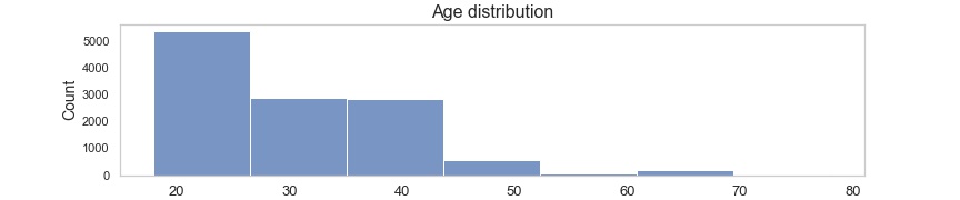
75% of customers are between age 18 and 38, median age 28.
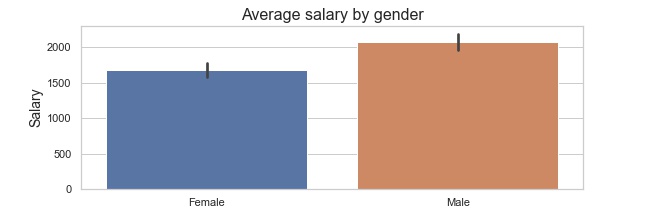
Difference in average salary by gender
Males: 2077.94 AUD, Females: 1679.37 AUD.
Average purchase transaction (POS transactions) amount is 39.8 AUD and every customer makes 27 of them on average every month.
Average week purchase volume and amount.
Average day purchase volume and amount.
Feature engineering
To understand our customer better, we will construct some new features that relate to their purchasing behaviours.
Create features like which state does the customer live in, how many purchases they make weekly, what is their average purchase amount, how many big purchases they make and what is their average balance.
customer_state = []
avg_weekly_purch_num = []
avg_weekly_trans_num = []
no_trans_days = []
avg_trans_amount = []
max_amount = []
num_large_trans = []
avg_trans_amount_overall = []
med_balance = []

for i in df['customer_id']:
    customer_state.append(customer_state_df[customer_state_df['id']==i]['state'].item())
    avg_weekly_purch_num.append(int(weekly_purch.loc[i]))
    avg_weekly_trans_num.append(int(weekly_trans.loc[i]))
    no_trans_days.append(pos_df[pos_df['customer_id']==i]['date'].nunique())
    avg_trans_amount.append(int(round(pos_df[pos_df['customer_id']==i]['amount'].mean(), 0)))
    max_amount.append(round(pos_df[pos_df['customer_id']==i]['amount'].max(), 1))
    num_large_trans.append(pos_df[(pos_df['customer_id']==i) & (pos_df['amount']>100)]['amount'].count())
    avg_trans_amount_overall.append(int(round(df[df['customer_id']==i]['amount'].mean(), 0)))
    med_balance.append(df[df['customer_id']==i]['balance'].median())

df['state'] = customer_state
df['avg_weekly_purch_num'] = avg_weekly_purch_num
df['avg_weekly_trans_num'] = avg_weekly_trans_num
df['no_trans_days'] = no_trans_days
df['avg_trans_amount'] = avg_trans_amount
df['max_amount'] = max_amount
df['num_large_trans'] = num_large_trans
df['avg_trans_amount_overall'] = avg_trans_amount_overall
df['med_balance'] = med_balance
Age bins
We will also bin the customer age to one four categories: below 20, between 20 and 40, between 40 and 60, over 60.
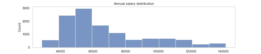
Annual salary for each customer
Find only salary payments.
df_salaries = df[df['txn_description']=='PAY/SALARY'].groupby('customer_id').sum()
Every customer in the dataset has a different frequency for receiving their salary, some get paid once a month, some every week. To find an average monthly salary we will sum up all their payments in the three months of data we have and divide it by three. To then get the annual salary we multiply the average monthly salary with 12.
annual_salaries = df_salaries['amount']/3*12 # annual salary for each customer
Predicting annual salary
First we will need to do some dummy encoding on categorical variables like ‘status’, ’txn_description’, ‘gender’, ‘state’ and ‘age_bin’.
Then check correlation between variabels and ‘annual_salary’.
num_feats.corr()['annual_salary'].sort_values(ascending=False)
annual_salary           1.000000
avg_trans_amount_ov     0.538656
med_balance             0.258076
balance                 0.257159
amount                  0.091111
avg_trans_amount        0.044312
num_large_trans        -0.045275
avg_weekly_trans_num   -0.079352
max_amount             -0.097739
no_trans_days          -0.172765
avg_weekly_purch_num   -0.189532
Name: annual_salary, dtype: float64
Here I realised avg_trans_amount_overall is suspiciously highly correlated. I decided to not use this as a feature for our predictive model because the calculation includes salary payments and we are trying to predict customers’ annual salary just by their purchasing behaviour, without knowing about their salary payments.
For testing, I chose to split our data to 70% train and 30% for test set.
Linear regression
Let’s build a simple linear regression model with sklearn to predict customers’ annual salary with features we defined earlier.
Our linear model valuation:
R-squared 0.5381890117545585
MAE: 13706.815968071387
MSE: 323705668.54002833
RMSE: 17991.822268464868
Plotting the predictions. Our model’s predictions are plotted in blue, perfect predictions in red.
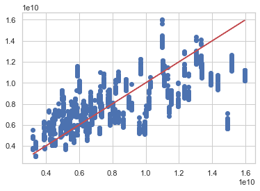
Our model’s predictions are kind of following the trend, but still too scattered to be trusted. So our linear regression model did not perform the best and this would not be an accurate way to predict customers’ annual salaries. But let’s try using a different model.
Gradient boosting
Gradient boosting is an ensemble learner. This means it will create a final model based on a collection of individual decision tree models.
Our gradient boosting model performed noticably better than the linear regression earlier:
R-squared 0.9842118273179078
MAE: 2476.2601909654327
MSE: 11066694.217258077
RMSE: 3326.66412750943
Plotting the predictions. Our gradient boosting model’s predictions are plotted in blue, perfect predictions in red.
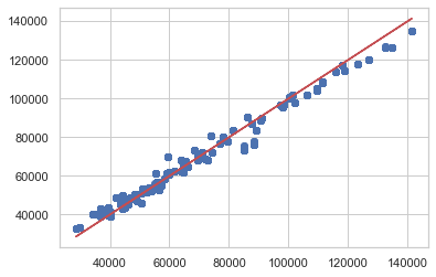
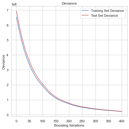
A gradient descent procedure is used to minimize the loss when adding trees. Our model’s loss is minimsed at around 400 trees.
Results
Our gradient boosting machine definitely outperformed the linear regression model. Should it be used to segment customers whose annual salary we do not have? Maybe not yet. We could definitely do better with more data (real data) and more parameter tuning.